Transformer neural net learns to run Conway's Game of Life just from examples

We find that a highly simplified transformer neural network is able to compute Conway’s Game of Life, just from being trained on examples of the game.

The simple nature of this model allows us to look at its structure and observe that it really is computing the Game of Life. It is not “just” a statistical model that predicts the most likely next state based on previous examples it’s seen — it learns to carry out the steps of the Game of Life algorithm: counting the number of neighbours, looking at the previous state of the cell, and using this information to determine the next state of the cell.

We observe that it learns to use its attention mechanism to compute 3x3 convolutions — 3x3 convolutions are a common way to implement the Game of Life, since it can be used to count the neighbours of a cell, which is part of the decision as to whether a cell lives or dies.

We refer to the model as SingleAttentionNet, because it consists of a single attention block, with single-head attention. The model represents a Life grid as a set of tokens, with one token per grid cell.

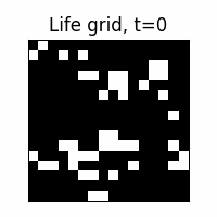
The following figure shows a Life game, computed by a SingleAttentionNet model:

The following figure shows examples of the SingleAttentionNet model’s attention matrix, over the course of training:

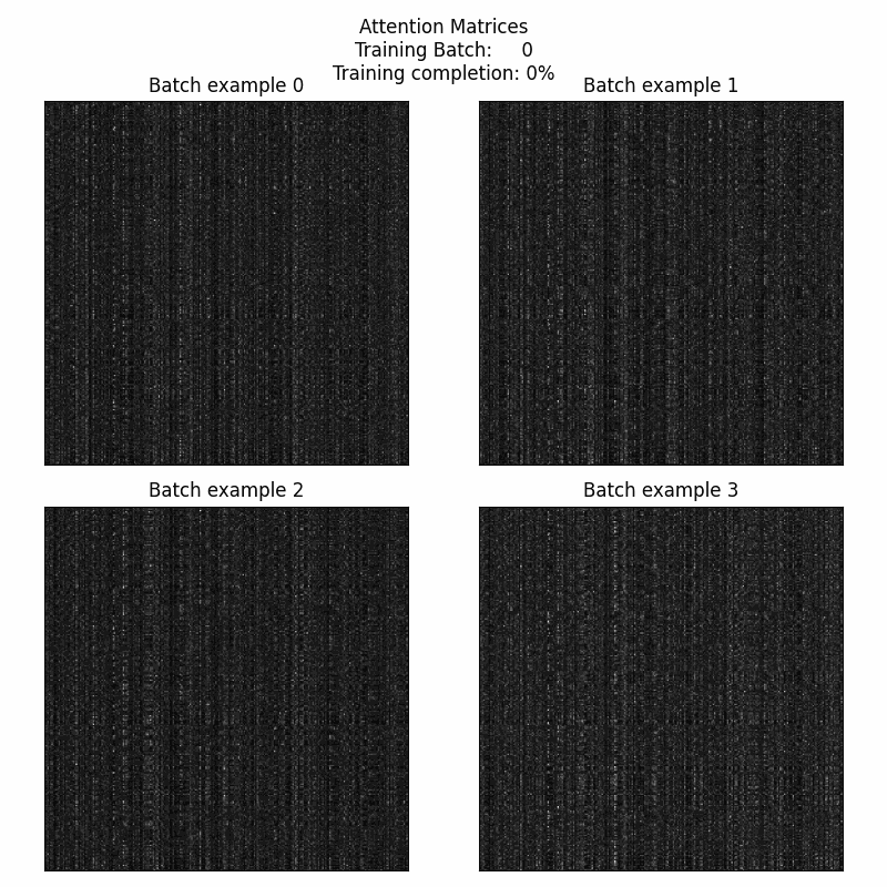
This shows the model learning to compute a 3 by 3 average pool via its attention mechanism, (with the middle cell excluded from the average).

Details

The code and model weights available, here.

The problem is modeled as:

model(life_grid) = next_life_grid

Where gradient descent is used to minimize the loss:

loss = cross_entropy(true_next_life_grid, predicted_next_life_grid)

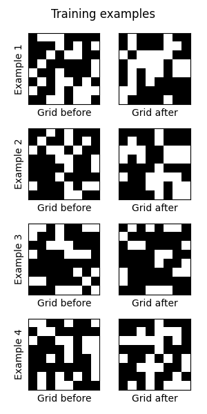
Life grids are generated randomly, to provide a limitless source of training pairs, (life_grid, next_life_grid). Some examples:

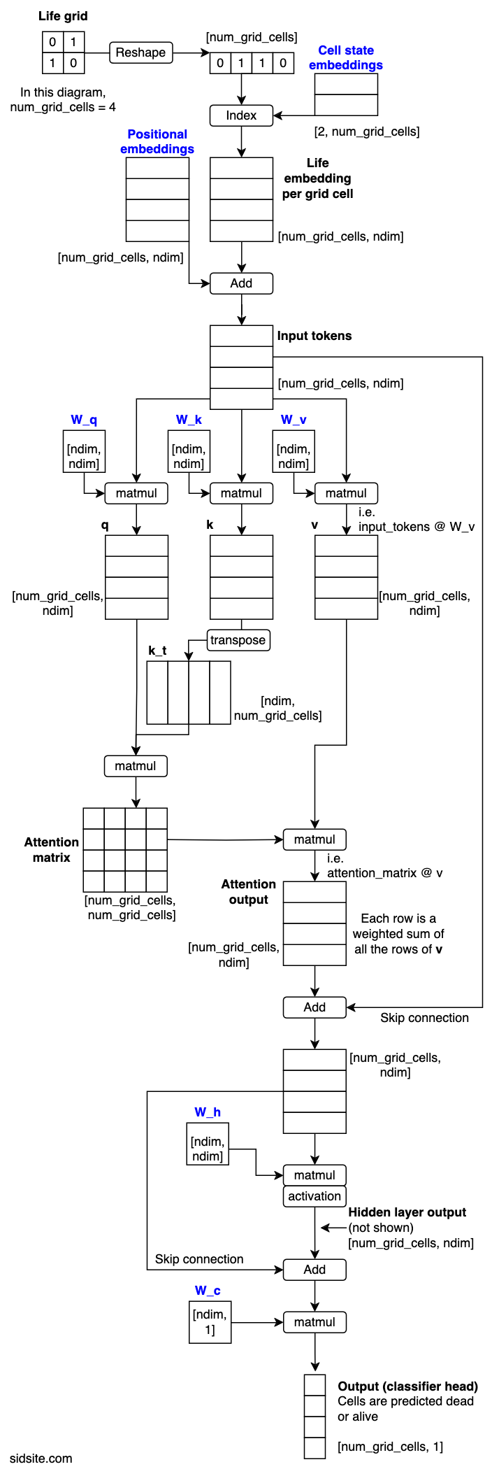
Model diagram

The model in the diagram processes 2-by-2 Life grids, which means 4 tokens in total per grid. Blue text indicates parameters that are learned via gradient descent. The arrays are labelled with their shape, (with the batch dimension omitted).

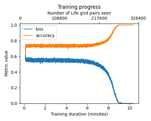
Training

On a GPU, training the model takes anywhere from a couple of minutes, to 10 minutes, or fails to converge, depending on the seed and other training hyperparameters. The largest grid size we successfully trained was 16x16.

Notes

The stopping condition for training was the model computing 10,000 training batches with perfect predictions. Since each batch contains 32 life grids the model has never seen before, that means it has predicted 32,000 life grid steps without making mistakes.

It was then further checked by running a further 10,000 randomly initialised life grids for 100 steps each. That’s 10,000 * 100 = 1,000,000 life grid steps computed correctly.

We found that it was enough to train the model on the first and second iterations of the random Life games, but it wasn’t enough to just train on the first iterations.

The model was fairly difficult to train - sensitive to hyperparameters and seed. Some seeds with the current hyperparameters don’t converge, (within a reasonable time frame to test them over). It also seems sensitive the software (or possibly hardware) environment, e.g. the current code runs reliably locally with the given seed, on a 3060 Ti GPU, but fails to run on a Google Colab T4 GPU instance.

We tried replacing the attention layer of the model with a manually computed Neighbour Attention matrix, and found the model learned the task far quicker, and generalised to arbitrary grid sizes. Not only this, but we checked that it computed every 3 by 3 subgrid correctly. Since the neighbour matrix means that only 3 by 3 subgrids are looked at by the classifier layer, there’s therefore no doubt that this instance of the model is “perfectly” computing Life.

We found that the same was true for replacing the layer with a 3-by-3 average pool.

Explanation of the model

A central finding of this work is that the SingleAttentionNet model doesn’t merely predict the next state of Conway’s Game of Life based on statistical patterns; it computes the Game of Life rules. This assertion is supported by several key observations:

Firstly, the model consistently achieves perfect accuracy (100%) when tasked with predicting the next state of entirely new, randomly generated Life grids, even over multiple steps. This high level of generalization strongly suggests it has learned the underlying rules rather than memorizing training examples.

Secondly, an examination of the model’s single attention block reveals its functional mechanism. As shown in the “attention matrix training” GIF above, the attention mechanism learns to perform a 3×3 averaging operation (excluding the center cell). This means that each token outputted from the attention layer contains just information about the 9 neighbours, as well as the cell itself due to the skip connection.

To confirm this, we conducted linear probe experiments, which demonstrated that the processed tokens encode this information, making the neighbor count and the cell’s prior state decodable.

Finally, these tokens are passed through a classifier layer. This layer, acting on the neighbor count and previous state information contained within each token, applies the Game of Life rules to determine the cell’s next state (alive or dead).

In essence, the SingleAttentionNet leverages its attention mechanism to gather local neighborhood information, encodes this information into its tokens, and then uses a simple classifier to apply the Game of Life rules to each cell independently, thereby simulating the game.

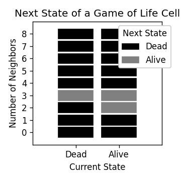
The rules of Life

Life takes place on a 2D grid with cells that are either dead or alive, (represented by 0 or 1). A cell has 8 neighbours, which are the cells immediately next to it on the grid.

To progress to the next Life step, the following rules are used:

• If a cell has 3 neighbours, it will be alive in the next step, regardless of it’s current state, (alive or dead).
• If a cell is alive and has 2 neighbours, it will stay alive in the next step.
• Otherwise, a cell will be dead in the next step.

These rules are shown in the following plot.

References:

• Springer et al - 2020 - It’s Hard For Neural Networks to Learn the Game of Life - https://arxiv.org/abs/2009.01398

• McGuigan - 2021 - Its Easy for Neural Networks To Learn Game of Life - https://www.kaggle.com/code/jamesmcguigan/its-easy-for-neural-networks-to-learn-game-of-life

• Vaswani et al - 2017 - Attention Is All You Need - https://arxiv.org/abs/1706.03762

• Conway’s Game of Life - https://en.wikipedia.org/wiki/Conway%27s_Game_of_Life

Citation:

@misc{radcliffe_life_transformer_2024,
  title={Training a Simple Transformer Neural Net on Conway's Game of Life},
  url={https://sidsite.com/posts/life-transformer/},
  howpublished={Main page: \url{https://sidsite.com/posts/life-transformer/}, GitHub repository: \url{https://github.com/sradc/life-transformer}},
  author={Radclffe, Sidney},
  year={2024},
  month={July}
}