Reverse-mode automatic differentiation from scratch, in Python
Automatic differentiation is the foundation upon which deep learning frameworks lie. Deep learning models are typically trained using gradient based techniques, and autodiff makes it easy to get gradients, even from enormous, complex models. ‘Reverse-mode autodiff’ is the autodiff method used by most deep learning frameworks, due to its efficiency and accuracy.
Let’s:
- Look at how reverse-mode autodiff works.
- Create a minimal autodiff framework in Python.
The small autodiff framework will deal with scalars. However we will look at a method of vectorising it with NumPy. We will also look at how to compute Nth order derivatives.
Note on terminology: from now on ‘autodiff’ will refer to ‘reverse-mode autodiff’. ‘Gradient’ is used loosely, but in this context generally means ‘first order partial derivative’.
How does autodiff work?
Let’s start with an example.
a = 4
b = 3
c = a + b  # = 4 + 3 = 7
d = a * c  # = 4 * 7 = 28
Q1: What is the gradient of $d$ with respect to $a$, i.e. $\frac{\partial{d}}{\partial{a}}$? (Go ahead and try this!)
Solving the ‘traditional’ way:
There’s many ways to solve Q1, but let’s use the product rule, i.e. if $ y = x_1x_2 $ then $y’ = x_1’x_2 + x_1x_2’$.
\[d = a * c\] \[\frac{\partial{d}}{\partial{a}} = \frac{\partial{a}}{\partial{a}} * c + a * \frac{\partial{c}}{\partial{a}}\] \[\frac{\partial{d}}{\partial{a}} = c + a * \frac{\partial{c}}{\partial{a}}\] \[\frac{\partial{d}}{\partial{a}} = (a + b) + a * \frac{\partial{(a + b)}}{\partial{a}}\] \[\frac{\partial{d}}{\partial{a}} = a + b + a * (\frac{\partial{a}}{\partial{a}} + \frac{\partial{b}}{\partial{a}})\] \[\frac{\partial{d}}{\partial{a}} = a + b + a * (1 + 0)\] \[\frac{\partial{d}}{\partial{a}} = a + b + a\] \[\frac{\partial{d}}{\partial{a}} = 2a + b\] \[\frac{\partial{d}}{\partial{a}} = 2*4 + 3 = 11\]Phew… and if you wanted to know $\frac{\partial{d}}{\partial{b}}$ you’d have to carry out the process again.
Solving the autodiff way
We’ll now look at the autodiff way to solve Q1. Here is a figure:
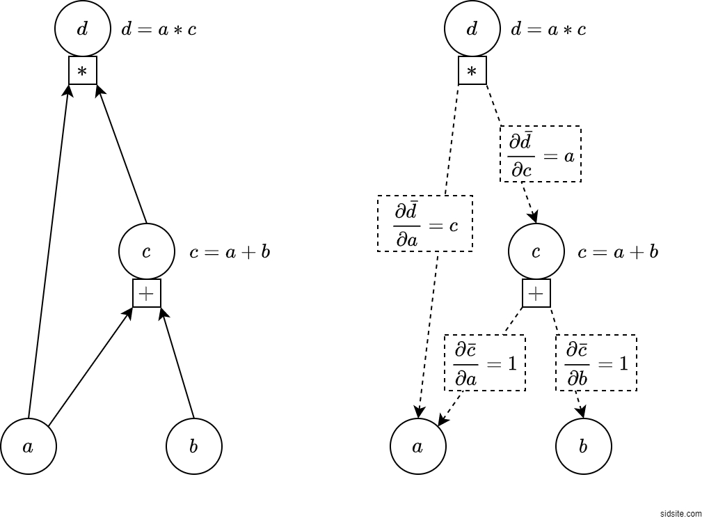
On the left we see the system represented as a graph. Each variable is a node; e.g. $d$ is the topmost node, and $a$ and $b$ are leaf nodes at the bottom.
On the right we see the system from autodiff’s point of view. Let’s call the values on the graph edges local derivatives. By using local derivatives and simple rules, we will be able to compute the derivatives that we want.
Here is the answer to Q1, calculated the autodiff way. Can you see how it relates to the figure?
\[\frac{\partial{d}}{\partial{a}} = \frac{\partial{\bar{d}}}{\partial{a}} + \frac{\partial{\bar{d}}}{\partial{c}} * \frac{\partial{\bar{c}}}{\partial{a}}\] \[\frac{\partial{d}}{\partial{a}} = c + a * 1\] \[\frac{\partial{d}}{\partial{a}} = a + b + a\] \[\frac{\partial{d}}{\partial{a}} = 2a + b\] \[\frac{\partial{d}}{\partial{a}} = 11\]We get this answer from the graph by finding the paths from $d$ to $a$ (not going against the dotted arrows), and then applying the following rules:
- Multiply the edges of a path.
- Add together the different paths.
The first path is straight from $d$ to $a$, which gives us the $\frac{\partial{\bar{d}}}{\partial{a}}$ term. The second path is from $d$ to $c$ to $a$, which gives us the term $\frac{\partial{\bar{d}}}{\partial{c}} * \frac{\partial{\bar{c}}}{\partial{a}}$.
Our autodiff implementation will go down the graph and compute the derivative of $d$ with respect to every sub-node, rather than just computing it for a particular node, as we have just done with $d$. Notice that we could compute the gradient of $d$ with respect to $c$, and $b$, without much more work.
Local derivatives
We saw ‘local derivatives’ on the graph edges above, written in the form: $ \frac{\partial \bar{y} }{\partial x}$.
The bar is to convey a simpler kind of differentiation.
In general: to get a local derivative, treat the variables going into a node as not being functions of other variables.
Note the distinction between local derivatives and partial derivatives: a partial derivative could take the whole graph into account, whereas a local derivative only looks at direct child nodes.
For example, recall that $d = a * c$. Then compare $ \frac{\partial{d}}{\partial{a}} = 2a + b $, to $ \frac{\partial \bar{d} }{\partial a} = c $. The local derivative $\frac{\partial \bar{d} }{\partial a} = c$, is obtained by treating $c$ as a constant before differentiating the expression for $d$.
Local derivatives make our lives easier.
It is often easy to define the local derivatives of simple functions, and adding functions to the autodiff framework is easy if you know the local derivatives. E.g.
Addition: $n = a + b$. The local derivatives are: $\frac{\partial \bar{n} }{\partial a} = 1$ and $\frac{\partial \bar{n} }{\partial b} = 1$.
Multiplication: $n = a * b$. The local derivatives are: $\frac{\partial \bar{n} }{\partial a} = b$ and $\frac{\partial \bar{n} }{\partial b} = a$.
Let’s create the framework
Overview of the implementation
A variable (or node) contains two pieces of data:
value- the value of the variable.local_gradients- the variable’s children and corresponding ‘local derivatives’.
The function get_gradients uses the variables’ local_gradients data to go through the
graph recursively*, computing the gradients.
(*I.e…
local_gradients contains references to child variables,
which have their own local_gradients,
which contain references to child variables,
which have their own local_gradients,
which contain references to child variables,
etc.)
The gradient of variable with respect to a child variable is computed using the rules we saw above:
- For each path from
variableto the child variable, multiply the edges of the path (givingpath_value). - Sum the path values.
… This gives the first order partial derivative of variable,
with respect to the child variable.
Implementing just enough to solve the example above:
from collections import defaultdict

class Variable:
    def __init__(self, value, local_gradients=()):
        self.value = value
        self.local_gradients = local_gradients

def add(a, b):
    "Create the variable that results from adding two variables."
    value = a.value + b.value
    local_gradients = (
        (a, 1),  # the local derivative with respect to a is 1
        (b, 1)   # the local derivative with respect to b is 1
    )
    return Variable(value, local_gradients)

def mul(a, b):
    "Create the variable that results from multiplying two variables."
    value = a.value * b.value
    local_gradients = (
        (a, b.value), # the local derivative with respect to a is b.value
        (b, a.value)  # the local derivative with respect to b is a.value
    )
    return Variable(value, local_gradients)

def get_gradients(variable):
    """ Compute the first derivatives of `variable`
    with respect to child variables.
    """
    gradients = defaultdict(lambda: 0)

    def compute_gradients(variable, path_value):
        for child_variable, local_gradient in variable.local_gradients:
            # "Multiply the edges of a path":
            value_of_path_to_child = path_value * local_gradient
            # "Add together the different paths":
            gradients[child_variable] += value_of_path_to_child
            # recurse through graph:
            compute_gradients(child_variable, value_of_path_to_child)

    compute_gradients(variable, path_value=1)
    # (path_value=1 is from `variable` differentiated w.r.t. itself)
    return gradients
Note: The recursive implementation of get_gradients is designed for clarity. For complex graphs (e.g. those with residual connections), this approach becomes inefficient due to traversing nodes multiple times, and it is better to iterate through a topologically sorted list. (I.e. it’s better to finish summing all the paths into a parent, before moving onto its children.)
Solving the example above:
a = Variable(4)
b = Variable(3)
c = add(a, b) # = 4 + 3 = 7
d = mul(a, c) # = 4 * 7 = 28

gradients = get_gradients(d)

print('d.value =', d.value)
print("The partial derivative of d with respect to a =", gradients[a])
d.value = 28
The partial derivative of d with respect to a = 11
Success!
Note we also get gradients for the other nodes:
print('gradients[b] =', gradients[b])
print('gradients[c] =', gradients[c])
gradients[b] = 4
gradients[c] = 4
Let’s take a look at the local_gradients values (the local derivatives):
print('dict(d.local_gradients)[a] =', dict(d.local_gradients)[a])
print('dict(d.local_gradients)[c] =', dict(d.local_gradients)[c])
print('dict(c.local_gradients)[a] =', dict(c.local_gradients)[a])
print('dict(c.local_gradients)[b] =', dict(c.local_gradients)[b])
dict(d.local_gradients)[a] = 7
dict(d.local_gradients)[c] = 4
dict(c.local_gradients)[a] = 1
dict(c.local_gradients)[b] = 1
We saw these in our example above as:
$ \frac{\partial \bar{d} }{\partial a} = c = 7$
$ \frac{\partial \bar{d} }{\partial c} = a = 4$
$ \frac{\partial \bar{c} }{\partial a} = 1$
$ \frac{\partial \bar{c} }{\partial b} = 1$
A few improvements
Let’s:
- Add a couple more functions.
- Enable the use of operators, such as +, *, - … using Python’s dunder (double underscore) methods.
class Variable:
    def __init__(self, value, local_gradients=[]):
        self.value = value
        self.local_gradients = local_gradients

    def __add__(self, other):
        return add(self, other)

    def __mul__(self, other):
        return mul(self, other)

    def __sub__(self, other):
        return add(self, neg(other))

    def __truediv__(self, other):
        return mul(self, inv(other))

def add(a, b):
    value = a.value + b.value
    local_gradients = (
        (a, 1),
        (b, 1)
    )
    return Variable(value, local_gradients)

def mul(a, b):
    value = a.value * b.value
    local_gradients = (
        (a, b.value),
        (b, a.value)
    )
    return Variable(value, local_gradients)

def neg(a):
    value = -1 * a.value
    local_gradients = (
        (a, -1),
    )
    return Variable(value, local_gradients)

def inv(a):
    value = 1. / a.value
    local_gradients = (
        (a, -1 / a.value**2),
    )
    return Variable(value, local_gradients)
Some more examples
We can get the gradients of arbitrary functions made from the functions we’ve added to the framework. E.g.
def f(a, b):
    return (a / b - a) * (b / a + a + b) * (a - b)

a = Variable(230.3)
b = Variable(33.2)
y = f(a, b)

gradients = get_gradients(y)

print("The partial derivative of y with respect to a =", gradients[a])
print("The partial derivative of y with respect to b =", gradients[b])
The partial derivative of y with respect to a = -153284.83150602411
The partial derivative of y with respect to b = 3815.0389441500993
We can use numerical estimates to check that we’re getting correct results:
delta = Variable(1e-8)
numerical_grad_a = (f(a + delta, b) - f(a, b)) / delta
numerical_grad_b = (f(a, b + delta) - f(a, b)) / delta
print("The numerical estimate for a =", numerical_grad_a.value)
print("The numerical estimate for b =", numerical_grad_b.value)
The numerical estimate for a = -153284.89243984222
The numerical estimate for b = 3815.069794654846
It’s easy to add more functions
You just need to be able to define the local derivatives.
import numpy as np

def sin(a):
    value = np.sin(a.value)
    local_gradients = (
        (a, np.cos(a.value)),
    )
    return Variable(value, local_gradients)

def exp(a):
    value = np.exp(a.value)
    local_gradients = (
        (a, value),
    )
    return Variable(value, local_gradients)

def log(a):
    value = np.log(a.value)
    local_gradients = (
        (a, 1. / a.value),
    )
    return Variable(value, local_gradients)
Let’s check that these work:
a = Variable(43)
b = Variable(3)
c = Variable(2)

def f(a, b, c):
    f = sin(a * b) + exp(c - (a / b))
    return log(f * f) * c

y = f(a, b, c)

gradients = get_gradients(y)

print("The partial derivative of y with respect to a =", gradients[a])
print("The partial derivative of y with respect to b =", gradients[b])
print("The partial derivative of y with respect to c =", gradients[c])
The partial derivative of y with respect to a = 60.85353612046653
The partial derivative of y with respect to b = 872.2331479536114
The partial derivative of y with respect to c = -3.2853671032530305
delta = Variable(1e-8)
numerical_grad_a = (f(a + delta, b, c) - f(a, b, c)) / delta
numerical_grad_b = (f(a, b + delta, c) - f(a, b, c)) / delta
numerical_grad_c = (f(a, b, c + delta) - f(a, b, c)) / delta

print("The numerical estimate for a =", numerical_grad_a.value)
print("The numerical estimate for b =", numerical_grad_b.value)
print("The numerical estimate for c =", numerical_grad_c.value)
The numerical estimate for a = 60.85352186602222
The numerical estimate for b = 872.232160009645
The numerical estimate for c = -3.285367089489455
That’s the end of our minimal autodiff implementation!
Of course there’s various features missing, such as:
- Vectorisation.
- Nth derivatives.
- Placeholder variables.
- Optimisations.
- The other great things deep learning / autodiff frameworks can do.
The following sections look at vectorisation and Nth derivatives.
A naive vectorisation
Let’s look at a computationally inefficient, but easy to implement, method of vectorising our autodiff framework.
The approach is:
- Put our
Variableobjects from above into NumPy arrays - We can then use NumPy operations
- That’s it..
import numpy as np

# convert NumPy array into array of Variable objects:
to_var = np.vectorize(lambda x : Variable(x))

# get values from array of Variable objects:
to_vals = np.vectorize(lambda variable : variable.value)
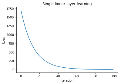
A single linear layer neural network (fitting noise to noise):
import matplotlib.pyplot as plt
np.random.seed(0)

def update_weights(weights, gradients, lrate):
    for _, weight in np.ndenumerate(weights):
        weight.value -= lrate * gradients[weight]

input_size = 50
output_size = 10
lrate = 0.001

x = to_var(np.random.random(input_size))
y_true = to_var(np.random.random(output_size))
weights = to_var(np.random.random((input_size, output_size)))

loss_vals = []
for i in range(100):
    y_pred = np.dot(x, weights)
    loss = np.sum((y_true - y_pred) * (y_true - y_pred))
    loss_vals.append(loss.value)
    gradients = get_gradients(loss)
    update_weights(weights, gradients, lrate)

plt.plot(loss_vals)
plt.xlabel("Time step")
plt.ylabel("Loss")
plt.title("Single linear layer learning")
plt.show()
Nth order derivatives
Note that enabling Nth order derivatives using reverse-mode autodiff is more costly computationally than only enabling first order derivatives. (Most deep learning frameworks only compute first order derivatives. Widely used optimisation methods, such as Adam, somewhat approximate higher order derivatives from the first order derivatives.)
We can enable our framework to compute Nth order derivatives by changing our get_gradient computations to use our Variable objects. This means that autodiff graphs will be created when computing derivatives, and we can then compute the derivatives of the derivatives that we are interested in with respect to the variables that we are interested in (and then the derivatives of derivatives, and derivatives of derivatives of derivatives, etc.).
The changes we will make are:
- To compute gradients using Variable objects.
- To change local_gradients to contain functions, instead of local gradient values.
A local_gradient function, multiply_by_locgrad, will multiply the path value that is passed to it with the local gradient value. This previously happened within the scope of get_gradients. However, since we are now defining local_gradients using our own Variable operations, we need to prevent infinite recursion (e.g. the local gradients of div are calculated using div, which would then compute more local gradients using div, which would then compute more local gradients using div, etc.) - using functions prevents this.
from collections import defaultdict

class Variable:
    def __init__(self, value, local_gradients=()):
        self.value = value
        self.local_gradients = local_gradients

    def __add__(a, b):
        return add(a, b)

    def __mul__(a, b):
        return mul(a, b)

    def __truediv__(a, b):
        return div(a, b)

# Useful constants:
ONE = Variable(1.)
NEG_ONE = Variable(-1.)

def add(a, b):
    value = a.value + b.value
    local_gradients = (
        # Note that local_gradients now contains lambda functions.
        (a, lambda path_value: path_value),
        # local gradient is 1, so multiply path_value by 1.
        (b, lambda path_value: path_value)
        # local gradient is 1, so multiply path_value by 1.
    )
    return Variable(value, local_gradients)

def mul(a, b):
    value = a.value * b.value
    local_gradients = (
        (a, lambda path_value: path_value * b),
        # local gradient for a is b, so multiply path_value by b.
        (b, lambda path_value : path_value * a)
        # local gradient for b is a, so multiply path_value by a.
    )
    return Variable(value, local_gradients)

def div(a, b):
    value = a.value / b.value
    local_gradients = (
        (a, lambda path_value : path_value * ONE/b),
        (b, lambda path_value : path_value * NEG_ONE * a/(b*b))
    )
    return Variable(value, local_gradients)

def get_gradients(variable):
    """ Compute the first derivatives of `variable`
    with respect to child variables.
    """
    gradients = defaultdict(lambda: Variable(0))

    def compute_gradients(variable, path_value):
        for child_variable, multiply_by_locgrad in variable.local_gradients:
            # "Multiply the edges of a path":
            value_of_path_to_child = multiply_by_locgrad(path_value)  # Now a function is used here.
            # "Add together the different paths":
            gradients[child_variable] += value_of_path_to_child
            # recurse through graph:
            compute_gradients(child_variable, value_of_path_to_child)

    compute_gradients(variable, path_value=ONE)  # Now path_value is a Variable.
    # (path_value=1 is from `variable` differentiated w.r.t. itself)
    return gradients
A bunch of examples:
"""
A 2nd derivative example.
y = x*x = x**2
y' = 2x (= 2*3 = 6)
y'' = 2
"""

x = Variable(3)
y = x * x

derivs_1 = get_gradients(y)
dy_by_dx = derivs_1[x]

print('y.value =', y.value)
print("The derivative of y with respect to x =", dy_by_dx.value)

derivs_2 = get_gradients(dy_by_dx)
dy_by_dx2 = derivs_2[x]
print("The 2nd derivative of y with respect to x =", dy_by_dx2.value)
y.value = 9
The derivative of y with respect to x = 6.0
The 2nd derivative of y with respect to x = 2.0
"""
2nd derivative of our original example.
d = a*(a + b)
d = a**2 + ab
dd_by_da = 2a + b (= 2*4 + 3 = 11)
dd_by_da2 = 2
"""

a = Variable(4)
b = Variable(3)
c = a + b # = 4 + 3 = 7
d = a * c # = 4 * 7 = 28

derivs_1 = get_gradients(d)
dd_by_da = derivs_1[a]

print('d.value =', d.value)
print("The partial derivative of d with respect to a =", dd_by_da.value)

derivs_2 = get_gradients(dd_by_da)
dd_by_da2 = derivs_2[a]
print("The 2nd partial derivative of d with respect to a =", dd_by_da2.value)
d.value = 28
The partial derivative of d with respect to a = 11.0
The 2nd partial derivative of d with respect to a = 2.0
"""
Another second derivative example, with division.
y = a*a/b
dy_by_da = 2*a/b (=2*3/7=0.8571...)
dy_by_da2 = 2/b (=2/7=0.2857...)
"""

a = Variable(3)
b = Variable(7)
y = a * a / b

derivs_1 = get_gradients(y)
dy_by_da = derivs_1[a]

print('y.value =', y.value)
print("The partial derivative of y with respect to a =", dy_by_da.value)

derivs_2 = get_gradients(dy_by_da)
dy_by_da2 = derivs_2[a]
print("The 2nd partial derivative of y with respect to a =", dy_by_da2.value)
y.value = 1.2857142857142858
The partial derivative of y with respect to a = 0.8571428571428571
The 2nd partial derivative of y with respect to a = 0.2857142857142857
"""
Nth derivative example
y = x**N
y' = N*x**(N-1) (=10*3**9=196830)
y'' = (N-1)*N*x**(N-2) (=9*10*3**8=590490)
y''' = (N-2)(N-1)*N*x**(N-3) (=8*9*10*3**7=1574640)
etc.
"""
from magic_timer import MagicTimer

N = 10
x = Variable(3)

y = ONE
for i in range(10):
    y *= x

print(f'At x={x.value}:\n')

target = y
for n in range(1,N+1):
    timer = MagicTimer()

    derivs_n = get_gradients(target)
    dy_by_dx_nth = derivs_n[x]
    target = dy_by_dx_nth

    print(f'The n={n} derivative of y w.r.t x is', dy_by_dx_nth.value)
    print('Elapsed time:', timer)
    print()
At x=3:

The n=1 derivative of y w.r.t x is 196830.0
Elapsed time: 693 microseconds

The n=2 derivative of y w.r.t x is 590490.0
Elapsed time: 6.3 milliseconds

The n=3 derivative of y w.r.t x is 1574640.0
Elapsed time: 13 milliseconds

The n=4 derivative of y w.r.t x is 3674160.0
Elapsed time: 360 milliseconds

---------------------------------------------------------------------------

RecursionError                            Traceback (most recent call last)
...
RecursionError: maximum recursion depth exceeded
"""
If we wanted very high order derivatives,
we could increase Python's recursion limit.
Alternatively, we could rewrite get_gradients,
so that the function doesn't recurse.
"""
import sys
print('Original recursion limit:', sys.getrecursionlimit())
sys.setrecursionlimit(10_000)
print('New recursion limit:', sys.getrecursionlimit())
Original recursion limit: 3000
New recursion limit: 10000
What’s next…
We can replace the scalars with NumPy arrays, creating a vectorised autodiff framework, suitable for training neural networks.
Check out my implementation here: https://github.com/sradc/SmallPebble.
References:
- Hands-On Machine Learning with Scikit-Learn and TensorFlow. A Géron, A. 2017
- https://en.wikipedia.org/wiki/Automatic_differentiation